Home
QGIS 5
Mapping Data Part 2: Chloropleth Maps
U.S. County-level Data
In the previous tutorial you experimented with the mapping of town population dataset by creating a points shapefile.
In this lesson you will display and map a polygon shapefile with county-level data for the United States in 1890.
I. Examine the Data
- In our shared folder find and open the census data csv for 1890 ("census1890_noNAs.csv").
- Examine the data. What kinds of variables (columns) are recorded in this dataset?
- What are the geographic units of analysis? (hint: look at the rows)
II. Import County Shapefile
- Open QGIS.
- Create a New Project, save it as "[yourName]_US"
- Keep the projection as "WGS 84" (EPSG: 4326).
- Open a base map (Web → QuickMapServices).
- Zoom into the United States and create a Spatial Bookmark to save this view
- There is a shapefile of U.S. County boundaries for 1890 in the shared folder ("counties1890.shp"). Open it in QGIS (Layers → Add Layer → Add Vector Layer).
- Adjust the symbology of the counties layer so that the fill is transparent and it looks something like this:

III. Import Census Data
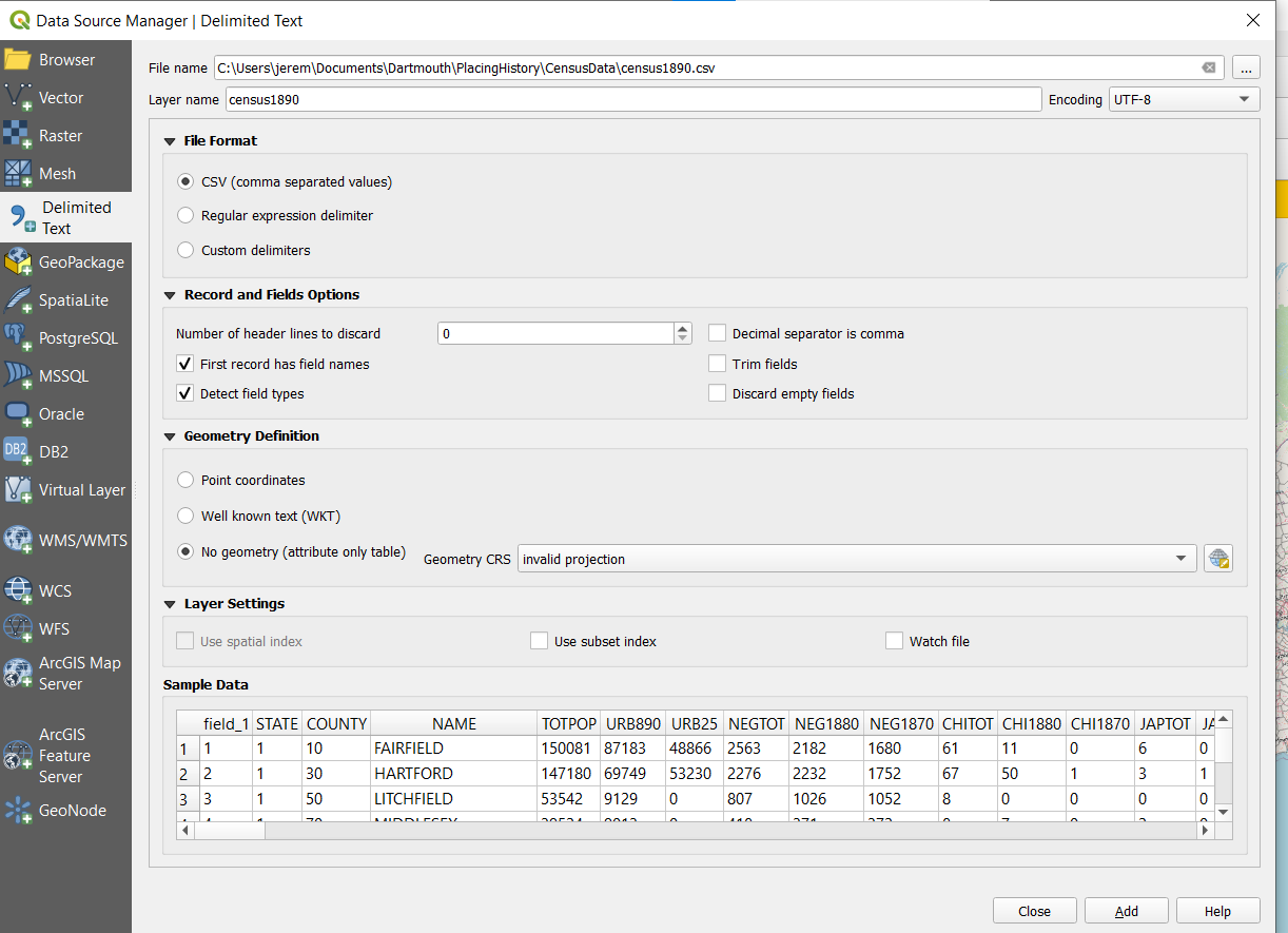
- Open the Census Data csv (Layer --> Add Layer --> Delimited Text Layer)
- *File Name*: Select the census data csv from the shared folder
- Make sure "No geometry" is selected. The window should look something like this:
- Press Add
- Note: the CensusData dataset should now appear in the Layers panel on the bottom left.
IV. Join Census Data with County shapefiles
The census dataset is not connected to any spatial data and therefore cannot be mapped. However, we can join the county-level census data with the county boundaries shapefile.
To join the dataset with the shapefile we need a common variable (column) by which to join the two tables. Since many counties in the U.S. have the same name we cannot join by county name.
Fortunately, both the dataset and the shapefile use a common identifier system to identify the counties known as "FIPS". We can then join the table and shapefile by:
- Right click on the counties shapefile and select Properties
- Select the Joins tab and select Add.
- In the Add Vector Join window:
- Join Layer: select "census1890".
- Join field: "FIPS"
- Target field: "FIPS"
- Press OK
- Press OK in the Layer Properties window
- To see if the Join was successful open the Attribute Table for the county shapefile (right-click → Open Attribute Table). Scroll right through the county shapefile. You should see the same variables (columns) found in the census dataset.
V. Display County-level population data
- Open the Symbology window for the county shapefile (right-click the shapefile → Properties → Symbology
- Select Graduated
- Select "totpop3" as your variable ("Value" menu)
- Select a Color Ramp of your choice.
- Experiment with different forms of breaking this total population data into Classes. You want to choose the right Mode that divides the data in a way that makes sense.
- Select OK
- What patterns do you notice in this data? What problems?
VI. Create a chloropleth map
- Here we will create a chloropleth map showing the Chinese-American population in the United States in 1890
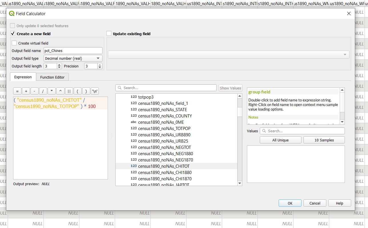
- NOTE: Chloropleth maps of population groups are more meaningful when they represent the percent of a population rather than a total number. For example, if you map the total number of "Chinese population" the Chinese and Chinese-American population will appear most prominently in urban counties with large populations. It is probably far more meaningful to map the Chinese-American population as a proportion or percent of the total population. Thus, you will need to create a new variable.
- To create this new variable, open the Attribute Table of the shapefile and use the Field Calculator to create a new variable (i.e. "pctChinese"). Then create a formula or "expression" for calculating the percent Chinese of the total population for the county. One way to create this new column is below:
- Return to your counties shapefile Properties window + Symbology tab. Now create a Graduated symbol representing the percent Chinese population.
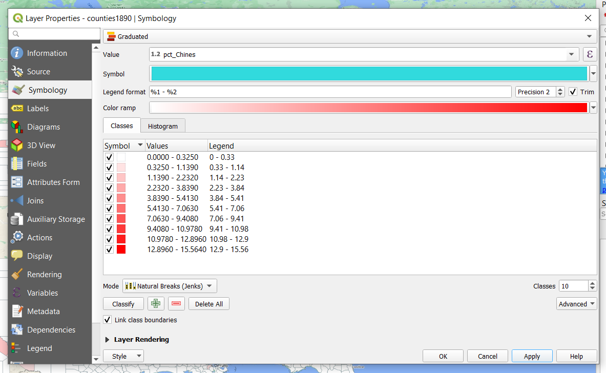
- Where was the Chinese-American population concentrated in 1890?
VII. Create your own chloropleth map
In this final step, you will choose your own census data variable to map. You will create a chloropleth map showing the spatial distribution of a particular variable across the country in 1890.
- Review the available data variables for the 1890 Census by opening the "02896-Codebook.pdf" document in the shared folder. Search in this document for 1890, and advance to page 149 in the codebook
- Review the available variables. Identify a variable from the 1890 census you would like to map.
- Following a similar procedure as you did for the Chinese-American population in 1890, create your chloropleth map
- Hint: If you want to keep your previous chloropleth map, you can right-click on your census data and duplicate the layer. Then for each variable you choose to map you can right-click on the duplicated layer go to the Source tab and change the "layer name" to indicate the data being mapped.
- Once complete and you are happy with it, submit it by placing it in the tutorial submissions folder as "qgis5_[yourname]".